Inferring Smooth Control:

Monte Carlo Posterior Policy Iteration with Gaussian Processes

Joe Watson & Jan Peters

Intelligent Autonomous Systems group, TU Darmstadt

joe@robot-learning.de

@JoeMWatson

Motivation

iCEM model predictive control
(Pinneri et al. 2020)

(this work)

Stochastic Search for Control

How do we preserve action correlations for smoothness?
Sample from the joint distribution! Fit the correlations!

$\va_t \sim p(\cdot)$

❗️$\mA \sim p(\cdot) = p(\va_1, \va_2, \dots)$❗️

$p(\va_1, \va_2, \dots) = \prod_t p(\va_t)$ 🚨

$q(\mA) = \sum_n w^{(n)} \delta(\mA - \mA^{(n)})$

❗️$ \min_{\color{#FF217D}{p}} \KL[q \mid\mid \color{#FF217D}{p}]$❗️

Posterior Policy Iteration

Optimizing for episodic return $R(\mA) = \E_{\vs_{t+1}\sim p(\cdot\mid\vs_t,\va_t),\,\vs_1\sim p(\cdot)}\left[\textstyle\sum_t r(\vs_t,\va_t)\right]$, what is $w^{(n)} = f(R^{(n)})$?

The objective $$ \textstyle\max_q \E_{\mA\sim p(\cdot)}\left[\alpha\,R(\mA)\right] - \KL[q(\mA)\mid\mid p(\mA)], $$

has a 'pseudo' (or Gibbs) posterior solution (e.g. Zellner (1998), Cantoni (2003)),

$$ q_\alpha(\mA) \propto \exp(\alpha R(\mA))\,p(\mA) \;\rightarrow\; w^{(n)}{\propto}\exp(\alpha R^{(n)}),\,\mA^{(n)}{\sim}p(\cdot). $$

$$ q_\alpha(\mA) \propto \exp(\alpha R(\mA))\,\color{blue}{p(\mA)}\;\rightarrow\; w^{(n)}{\propto}\exp(\alpha R^{(n)}),\,\mA^{(n)}{\sim}p(\cdot). $$

$$ q_\color{#FF217D}{\alpha}(\mA) \propto \exp(\color{#FF217D}{\alpha} R(\mA))\,\color{blue}{p(\mA)}\;\rightarrow\; w^{(n)}{\propto}\exp(\color{#FF217D}{\alpha} R^{(n)}),\,\mA^{(n)}{\sim}p(\cdot). $$

Posterior policy iteration (PPI): pseudo-posteriors for optimal control (Rawlik et al. (2013)).

Research questions:

$ \color{blue}{\text{1) How to design the prior for control?}} $

$ \color{#FF217D}{\text{2) How to set the temperature for Monte Carlo optimization?}} $

Action Priors for Control

For robotics, IID noise is not desirable for physical systems!

Jerky movements will damage a physical system and environment
Desirable solutions, like humans, typically move smoothly

Action Priors for Control

Action smoothing is often an implementation detail, rather than theory (Williams et al. 2018, Nagabandi et al. 2019, Pinneri et al. 2020, ...).

E.g. first-order smoothing: $ \beta\,\va_t^{(n)} + (1-\beta)\,\va_{t-1}^{(n)} $

Desiderata

Ensure the solution is sufficiently smooth...
...without introducing lag.
Smooth exploratory samples for Monte Carlo efficiency.

Action Priors for Control

Nonparametric Gaussian processes (GP) (Rasmussen & Williams, 2006) capture a diverse range of smoothed stochastic processes.

$$p(a_1, a_2, \dots) = \gN(\mathbf{0}, \mSigma) = \gG\gP(0, \gC(\vt)),\, \vt = [t_1, t_2, \dots]$$

Vector-valued Gaussian Processes

How can we scale nonparametric GPs to high-dimensional action sequences? $$ \mA \in \mathbb{R}^{H \times d_a} $$

A Matrix Normal Distribution

For a random matrix $\mX \in \sR^{n\times p}$, it follows a matrix normal distribution $\mX{\,\sim\,}\gM\gN(\mM, \mK, \mSigma)$, where $$ p(\mX) = \gM\gN(\mX;\mM, \mK, \mSigma) = \frac{1}{(2\pi)^{np/2}|\mK|^{p/2}|\mSigma|^{n/2}}\exp\left(-\frac{1}{2}\text{tr}\{\mSigma^{-1}(\mX-\mM)\tran\mK\inv(\mX-\mM)\}\right), $$ for $\mM\in\sR^{n\times p}, \mK\in \sR^{n\times n}, \mK \succcurlyeq 0$ and $\mSigma\in \sR^{p\times p}, \mSigma \succcurlyeq 0$, if and only if $\text{vec}(\mX){\,\sim\,}\gN(\text{vec}(\mM), \mSigma\otimes\mK)$, where $\otimes$ denotes the Kronecker product.

$$ \text{Kronecker product: }\; \begin{bmatrix} \Sigma_{11} & \dots &\Sigma_{1m} \\ \vdots & \ddots & \vdots \\ \Sigma_{n1} & \dots &\Sigma_{nm} \end{bmatrix} \otimes\mK = \begin{bmatrix} \Sigma_{11}\,\mK & \dots &\Sigma_{1m}\,\mK \\ \vdots & \ddots & \vdots \\ \Sigma_{n1}\,\mK & \dots &\Sigma_{nm}\,\mK \end{bmatrix} \quad \text{(covariance of flattened matrix)} $$

Define our action prior,
$$ \mA = [\va_t,\va_{t+1},\dots,\va_{t+1}] \sim \gM\gN(\vzero, \gK(\vt), \mSigma), \quad \vt = [t, t+\Delta, \dots, t+H\Delta], $$ for covariance function $\gK(t,t')$, timestep $\Delta$ and horizon $H$.

Continuous-time Gaussian Processes

How do we update our solution each time step for model predictive control?

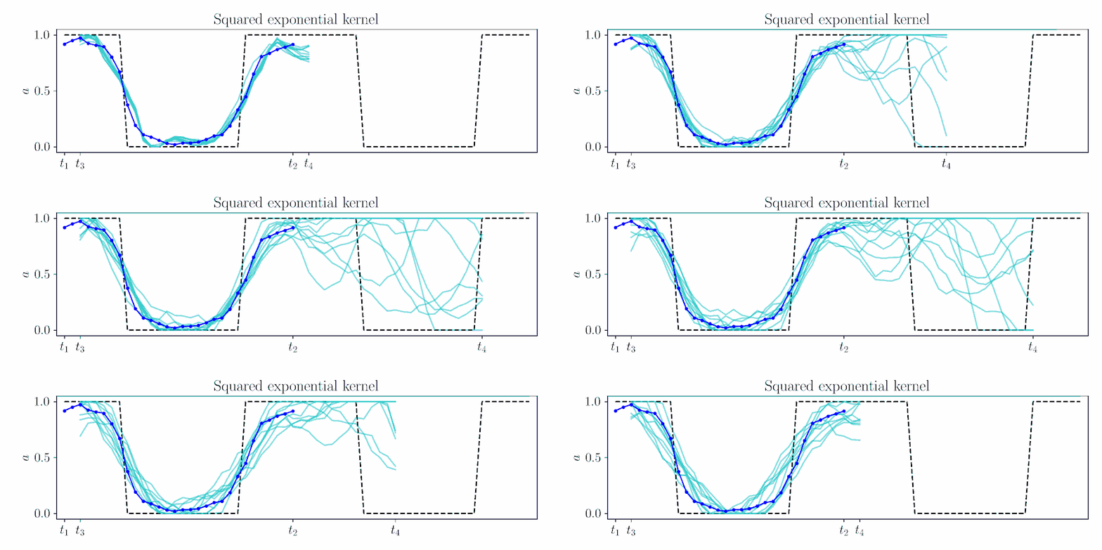
Gaussian processes provide an elegant means to 'time shift' in MPC.

Plan for timesteps $t$ to $t+H$, based on previous solution up to time $\tau$, $$ q_\alpha(\va_{t:t+H}\mid \gO_{1:\tau}) = \textstyle\int q_\alpha(\va_{1:t+H}\mid\gO_{1:\tau})\,\mathrm{d}\va_{1:t} \propto \textstyle\int \underbrace{p(\gO_{1:\tau}\mid\va_{1:\tau})}_{\text{previous solution}}\, \underbrace{p(\va_{1:t+H})}_{\text{time-extended prior}} \, \mathrm{d}\va_{1:t}. $$

The previous solution is due to an unknown likelihood $\color{blue}{\gN(\vmu_{\gO|t_1:t_2}, \mSigma_{\gO|t_1:t_2})}$,
$ \vmu_{t_1:t_2|\gO} = \vmu_{t_1:t_2} + \mK_{t_1:t_2}(\color{blue}{\vmu_{\gO|t_1:t_2}}-\vmu_{t_1:t_2}) ,\quad \mSigma_{t_1:t_2, t_1:t_2|\gO} = \mSigma_{t_1:t_2,t_1:t_2}- \mK_{t_1:t_2}\color{blue}{\mSigma_{\gO|t_1:t_2}}\mK_{t_1:t_2}\tran, $
where $\mK_{t_1:t_2}{\,=\,}\mSigma_{t_1:t_2, t_1:t_2} \color{blue}{\mSigma_{\gO|t_1:t_2}}\inv$.

Compute unknown terms using old posterior and prior,
$\color{magenta}{\vnu_{t_1:t_2}} = \color{blue}{\mSigma_{\gO|t_1:t_2}}\inv(\color{blue}{\vmu_{\gO|t_1:t_2}}-\vmu_{t_1:t_2}) = \mSigma_{t_1:t_2, t_1:t_2}\inv(\vmu_{t_1:t_2|\gO} - \vmu_{t_1:t_2}) $,
$\color{magenta}{\mathbf{\Lambda}_{t_1:t_2}} = \color{blue}{\mSigma_{\gO|t_1:t_2,t_1:t_2}}\inv = \mSigma_{t_1:t_2,t_1:t_2}\inv(\mSigma_{t_1:t_2,t_1:t_2} - \mSigma_{t_1:t_2,t_1:t_2|\gO})\mSigma_{t_1:t_2,t_1:t_2}\inv $.

Combine these likelihood terms with the time-shifted prior $\color{turquoise}{\gN(\vmu_{t_3:t_4}, \mSigma_{t_3:t_4})}$ and cross-correlation $\color{SeaGreen}{\mSigma_{t_3:t_4,t_1:t_2}} = k(\vt_{t_3:t_4},\vt_{t_1:t_2})$
$\vmu_{t_3:t_4|\gO} = \color{turquoise}{\vmu_{t_3:t_4}} + \color{SeaGreen}{\mSigma_{t_3:t_4,t_1:t_2}} \color{magenta}{\vnu_{t_1:t_2}},$
$\mSigma_{t_3:t_4,t_3:t_4|\gO} = \color{turquoise}{\mSigma_{t_3:t_4,t_3:t_4}} - \color{SeaGreen}{\mSigma_{t_3:t_4,t_1:t_2}} \color{magenta}{\mathbf{\Lambda}_{t_1:t_2}} \color{SeaGreen}{\mSigma_{t_3:t_4,t_1:t_2}}\tran.$

Experimental Results

PPI model predictive control
(this work)

Experimental Results

Dirty Laundry 🧺🤢

Gaussian processes introduce implementation complexity and some numerical sensitivity.
Gaussian processes introduce hyperparameters (e.g. lengthscales) tuned offline.
Smoothness (i.e. lengthscales) cannot always be learned from expert demonstrations.

Inferring Smooth Control:
Monte Carlo Posterior Policy Iteration with Gaussian Processes

Joe Watson, Jan Peters

Intelligent Autonomous Systems group, TU Darmstadt

joe@robot-learning.de @JoeMWatson joemwatson.github.io

Poster: OGG (260), Level 0 Room 038
Paper: arxiv.org/abs/2210.03512
Code: github.com/JoeMWatson/monte-carlo-posterior-policy-iteration
Slides: joemwatson.github.io/slides/corl22oral
Website: monte-carlo-ppi.github.io

Posterior Constraints for Monte Carlo Optimization

$$ q_\color{#FF217D}{\alpha}(\mA){\,\propto\,}\exp(\color{#FF217D}{\alpha} R(\mA))\,p(\mA). $$ Choose $\color{#FF217D}{\alpha}$ to balance greediness and inference quality?

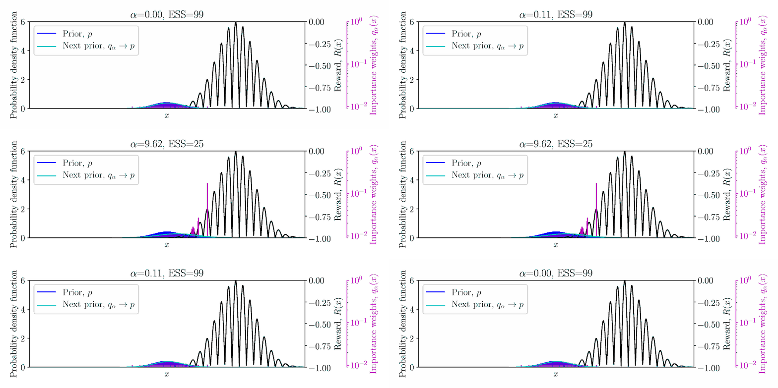
Posterior Constraints for Monte Carlo Optimization

Three ways to derive the pseudo-posterior $ q_\alpha(\mA){\,\propto\,}\exp(\alpha R(\mA))\,p(\mA): $

1) Gibbs likelihood, $\hspace{12.9em}\max_q \E_q[R] - \frac{1}{\alpha}\KL[q\mid\mid p]$.

2) Relative entropy policy search (REPS) (Peters et al.), $\max_q \E_q[R] \; \text{s.t.} \; \KL[q\mid\mid p] \leq \epsilon$.

3) Minimum KL problem (this work), $\hspace{6.3em} \min_q \KL[q \mid \mid p] \; \text{s.t.} \; \E_q[R] = R^*$.

$E_q[R]$ is approximated using importance sampling!

Lower-bound Policy Search (LBPS). Maximize $R^*$ using a probabilistic lower-bound of $\E_q[R]$,
$$ \max_\alpha \hat{R}^*_\alpha = \max_\alpha \E_{q_\alpha \, / p}[R(\mA)] - ||R||_\infty\sqrt{\frac{1-\color{#FF217D}{\delta}}{\color{#FF217D}{\delta}}\frac{1}{\color{blue}{\hat{N}_\alpha}}}, \quad \text{where $\color{blue}{\hat{N}_\alpha}$ is the effective sample size}. $$ we balance optimization with inference accuracy through bound probability $\color{#FF217D}{\delta} \in [0, 1]$.